Network Tomography Definition
Network tomography is the inference of the internal behavior and topology of a network, based on end-to-end network measurements. Imagine having the ability to probe the network from its edges and reach conclusions about its guts. Similarly, computer tomography allows you to create an image of an object or a human body by sending x-rays. In both cases tomography is a minimally invasive method that enables the creation of an image of the internals of a system or object without physical access to it.
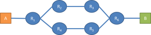
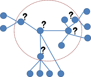
On first thought it sounds like a very interesting idea: “What if I run a certain number of traceroute commands from several different edges of the network, and by sorting through the results I infer what the topology looks like?” However, very quickly you realize that not all routers respond to traceroute (you will have partial information), the routing might change between two different commands (your results will vary with time), and then you have to decide which edges to use for the traceroute. For example, you might have a network that looks like this:
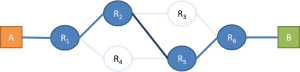
But the information collected by traceroute leads you to believe that it looks like this:
Then, after you infer the topology, you start thinking about other interesting stuff you could do with network tomography. “What if I could know which nodes are dropping packets and causing delays?” “How routing changes with respect to time?” You can argue that there are other ways to know this information, such as making actual measurements at each node with OpenFlow or have a passive device for deep packet inspection. Well, these options are feasible only when you have access to the internals of the network. Network tomography would be useful if you wanted to map and monitor a network without having any access to its internal details. A good example would be of, say, ISP Acme, which needs to deliver traffic through a peer ISP Corp, and Acme needs to know when Corp is responsible for congestion and performance problems experienced by Acme’s customers. In this case, Acme doesn’t have any formal access to Corp’s network topology and performance, so it can only infer this data through probing.
These two examples both show how useful network tomography can be, but also how difficult of a problem it is. The term and idea of network tomography dates back to 1996 in the paper by Y. Vardi [1]. Since then the academic bibliography has been very active, but there haven’t been major breakthroughs and wide adoption in the industry. This paints the picture of how challenging and difficult of a problem it is.
In this blog I’ll give a few examples and basic ideas behind network tomography because I find it a very interesting idea with great potential. However, tackling this problem is not for the faint of heart. It requires a blend of advanced knowledge in statistics, math, computer science, and networking. On top of that, applying network tomography on very large networks might create substantial traffic overhead and can become computationally intractable.
There are different types of tomography depending on the way information is collected and what type of network information is sought.
Passive vs. Active Tomography
Active tomography is based on probing a network by generated traffic. This method gives the flexibility to generate exactly the packets needed for each task, and it doesn’t require access to any internal network nodes. However, it creates extra traffic on the network, which might be substantial in some cases.
Passive tomography is based on capturing real traffic that is generated by users. In this case, you need access to the edge routers of the network. The benefit is that you don’t need to overload the network with extra traffic, and it is based on real user traffic.
Unicast vs. Multicast Traffic
In terms of the types of packets used, we differentiate between unicast and multicast tomography. Unicast measurements are not as accurate as multicast, but since many networks don’t support multicast forwarding we need to work with unicast tomography. When we need to send a probing packet to a single destination, unicast tomography is the best option. In the examples below, we see how the two types of packets can be used and how they compare.
Use Cases
The three uses cases below demonstrate some basic ideas of network tomography. As you can see, the examples are simple and we make certain assumptions about the network and the probing packets. Real networks are far more complex and there are many uncertainties that we would have to deal with.
1) Infer logical topology with traceroute
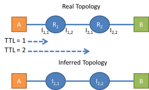
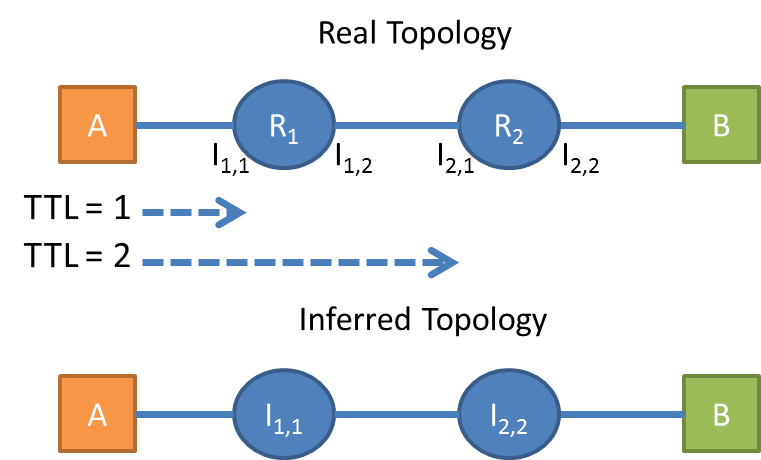
Traceroute is very useful when we want to see a hop-by-hop route of a packet, from a source to a destination. This is possible only when all routers cooperate and respond to traceroute requests. And even if they do, we see only the addresses of the interfaces and not the routers themselves. In the figure below we infer that from A to B there are two routers, R1 and R2, with interfaces I1,1 and I2,1.
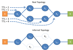
Below is a bit more complex example that shows the limitations of this method. The three packets follow divergent flows and the inferred topology does not match the structure of the real one.
2) Calculate loss rate
In this use case, we assume that we know the topology of the network and we want to calculate the probability for each router to drop a packet. The basic idea is pretty straightforward. Suppose that we send a multicast packet from A to reach two end nodes with the assumption that the paths traversed by the packets share some common sub-path and then diverge at some point. Let’s take as an example the topology below.
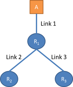
For a multicast packet sent from A to R2 and R3 there are four outcomes as shown in the table.
| R2 | R3 | Conclusion |
| No losses | ||
| Loss occurred on link 2 | ||
| Loss occurred on link 3 | ||
| Loss might have occurred on links 1 or 2 and 3 (inconclusive) |
If we run this experiment repeatedly the rate of losses on links 2 and 3 can be calculated. The number of the packets that reach both R2 and R3 and the packets that reach only R2 gives the loss rate on link 3 as follows:
Loss(Link 3) = 1 – (# of packets reaching both R2 and R3) / (# packets reaching only R2).
Similarly, you can calculate the loss rate for link 2. If multicast forwarding is not an option, then we can send unicast back-to-back packet pairs with destinations R2 and R3. However, this means that the packets might reach the nodes at different times and the path between the probes may change to a more complicated topology.
3) Delay distributions
In this case we want to estimate the delay of a specific link. We assume that we know the topology of the network and that there is a certain minimum propagation delay along each link which we also know. Let’s take the same topology we used in the previous use case with minimum propagation delays dMin,link1, d Min,link2, and d Min,link3 as an example. The tomography consists of sending multicast packets from A to nodes R2 and R3 and measuring the delay to reach each node. The delay on link 1 is identical for both packets, and any difference in the two delays is due to differences in links 2 and 3. If the arrival time to link 2, tlink2, is equal to the minimum possible delay this means that the delay on link 1 was the minimum possible one, and after the packet split at R1 the delay on link 3 is equal to:
dlink3 = tlink3 – d Min,link1.
Repeating this experiment multiple times allows us to make a good estimate of the delay on links 2 and 3.
Now try to apply these use cases to a network that is a bit more complex and looks like this:
Conclusion
You can quickly understand how difficult network tomography becomes as the complexity of the network increases. Nonetheless, it is an active research field in academia and the interested reader can find lots of material online. Some references that have been used in this blog and you might find useful are the following:
[1] Y. Vardi, Network Tomography: Estimating Source-Destination Traffic Intensities from Link Data, Journal of the American Statistical Association, March 1996.
[2] M. Coates, A. O. Hero III, R. Nowak, and B. Yu, Internet Tomography, IEEE Signal Processing Magazine, May 2002.
[3] R. Teixeira, Making Network Tomography Practical, Laboratoire LIP6 CNRS and UPMC Paris Universitas, 2009.
[4] P. Qin, B. Dai, B. Huang, G. Xu, and K. Wu, A Survey of Network Tomography with Network Coding, Cornel University, 2014.


